Background information about the checks
Porosity check
Potential porosity is thought to be a key defining criterion for MOFs. For assembling the widely used CoRE-MOF database (see first and second paper) Yongchul G. Chung et al. used a pore limiting diameter (PLD) of more than 2.4 Å (approximately the van der Waals diameter of a hydrogen molecule) as threshold for the distinction of porous and non-porous (or nanoporous) MOFs.
In mofchecker, we follow this definition and use zeopp with the high-accuracy flag and the default atom radii to compute the largest free sphere. If it is above or equal to 2.4 Å the :py:attr`~mofchecker.MOFChecker.is_porous` will return True.
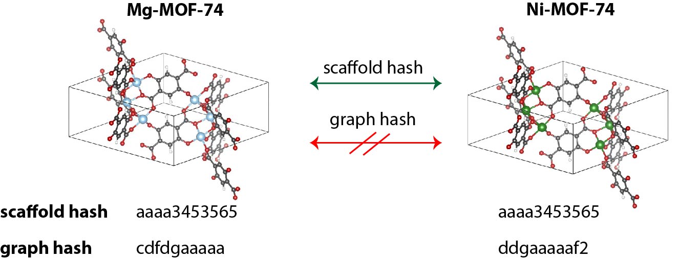
Graph hash and scaffold hash
For a given MOF structure
the scaffold hash (
scaffold_hash) is unique for a given connectivity (bond network), independent of the atomic species in the graphthe structure graph hash (
graph_hash) is like the scaffold hash, but also considers the atomic elements (nodes) in the graph
What is it useful for?
The scaffold and structure graph hashes allow to quickly identify duplicates in large structure databases.
The concept of duplicate structures, as defined by comparing their graph_hash, closely follows the one proposed by Barthel et al. :
[…], from a MOF point of view two structures are considered identical if they share the same bond network, with respect to the atom types and their embedding: i.e., if two structures can in principle be deformed into each other without breaking and forming bonds.
The scaffold hash can be useful to find families of related MOFs. For example, all members of the (unfunctionalized) MOF-74 family, such as Ni-MOF-74 or Mg-MOF-74, group under the same hash.
How does it work?
mofchecker
reduces the structure to the primitive cell using pymatgen and spglib (use
primitive=Falseto disable this)analyzes the bonding network and creates a corresponding structure graph using pymatgen (use
_set_cnn()to switch to a different bond analysis method).computes the Weisfeiler-Lehman hash of the structure graph using networkx.
The Weisfeiler Lehman algorithm is explained in the English translation of the original paper and a popular blog post. The figure below (adopted from Michael Bronstein’s blog) illustrates the concept:
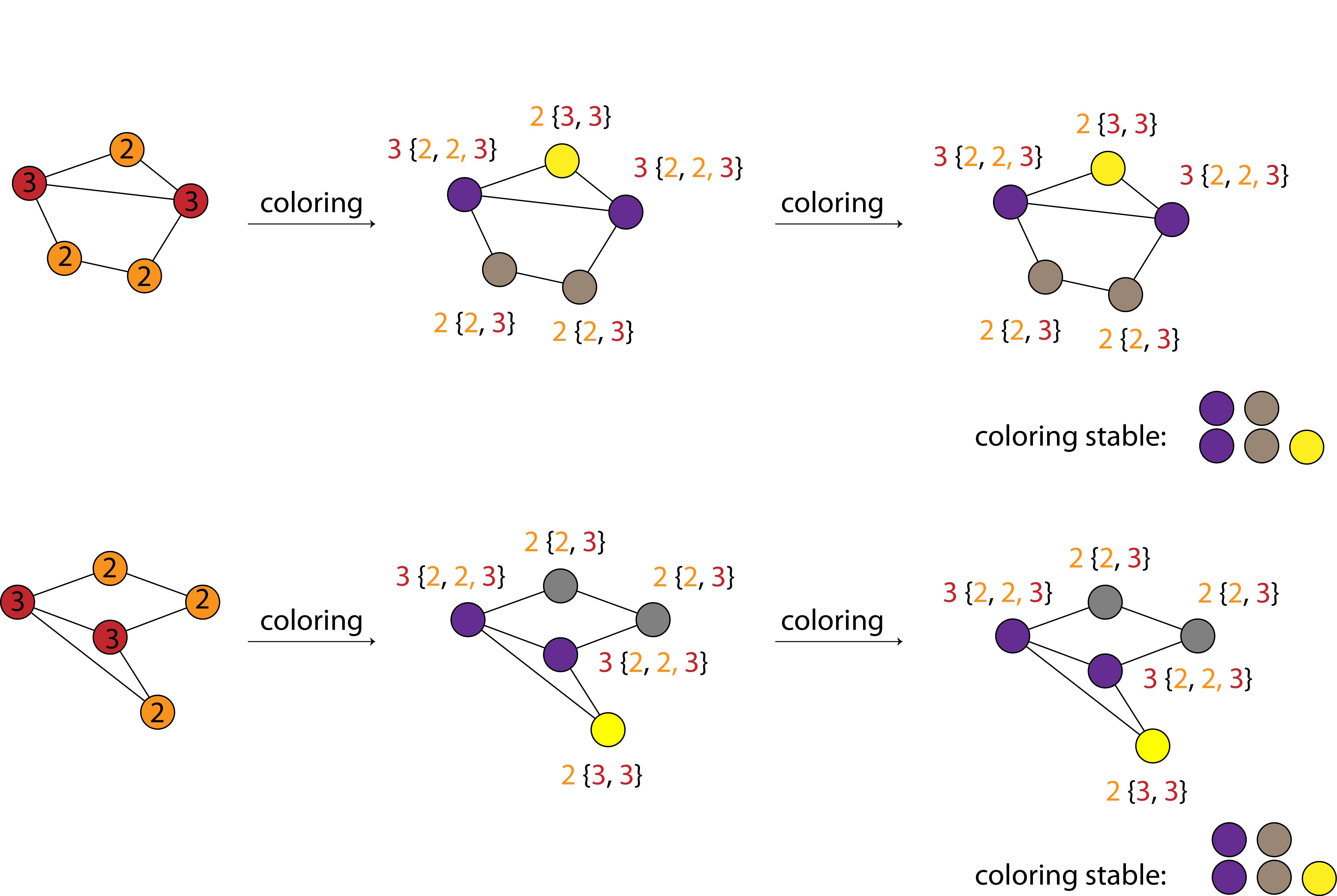
Briefly:
Start by labelling each atom (node) with its atomic number (graph_hash) or the number of its connected neighbors (scaffold_hash).
Extend the labels with the labels of the nearest neighbors. Color nodes according to their labels.
Continue until coloring converges or the maximum number of iterations is reached (we find that 3rd-nearest neighbors is enough)
Create a histogram of colors of all nodes and return a (ideally unique) hash of it.
What can go wrong?
Hashes of two structures may differ unexpectedly if
The two structures were not reduced to the same primitive cell. This can happen when the symmetry in one of the structures is broken.
The bonding network of the two structures is not the same. Bonds between atoms are assigned based on heuristics; you may want to try a different method using
_set_cnn().
It is also possible (but unlikely) that the hashes of two structures coincide unexpectedly if
there is an unlucky hash clash. Weisfeiler Lehman has some edge cases)